
Bibliographic Info
- 저자: Chih-Kai Yang, Neo Ho, Yi-Jyun Lee, Hung-yi Lee
- 연도: 2025
- 제목: AudioLens: A Closer Look at Auditory Attribute Perception of Large Audio-Language Models
- 학회/저널: arXiv preprint arXiv:2506.05140v2 (2025년 8월 24일), National Taiwan University,
Abstract
Abstract—Understanding the internal mechanisms of large audiolanguage models (LALMs) is crucial for interpreting their behavior and improving performance. This work presents the first in-depth analysis of how LALMs internally perceive and recognize auditory attributes. By applying vocabulary projection on three state-of-the-art LALMs, we track how attribute information evolves across layers and token positions. We find that attribute information generally decreases with layer depth when recognition fails, and that resolving attributes at earlier layers correlates with better accuracy. Moreover, LALMs heavily rely on querying auditory inputs for predicting attributes instead of aggregating necessary information in hidden states at attribute-mentioning positions. Based on our findings, we demonstrate a method to enhance LALMs. Our results offer insights into auditory attribute processing, paving the way for future improvements. Index Terms—Large audio-language model, auditory attribute perception, internal mechanism, interpretability.
I. INTRODUCTION
기존 LALM 모델 논문 리스트
| 구분 | 논문 제목 | 링크 | 주요 주제 |
| 1 | Listen and Speak Fairly: A Study on Semantic Gender Bias in Speech Integrated Large Language Models (Lin et al., 2024) | arXiv 2407.06957 | Semantic Gender Bias in Speech-Integrated LLMs |
| 2 | The Curse of Multi-Modalities: Evaluating Hallucinations of Large Multimodal Models Across Language, Visual, and Audio (Leng et al., 2024) | arXiv 2410.12787 | Hallucinations in LMMs |
| 3a | Transformer Feed-Forward Layers Build Predictions by Promoting Concepts in the Vocabulary Space (Geva et al., 2022) | arXiv 2203.14680 | Transformer FFN 내부 동작 해석 (“Concept Promotion”) |
| 3b | Jump to Conclusions: Short-Cutting Transformers With Linear Transformations (Din et al., 2023) | arXiv 2303.09435 | Training-Free Vocabulary Projection / Linear Shortcut |
Transformer 중간 해석
Interpreting GPT: the logit lens
the logit lens : Report review
interpreting GPT: the logit lens — LessWrongThis post relates an observation I've made in my work with GPT-2, which I have not seen made elsewhere. …www.lesswrong.com 준비중
moos-tudy.tistory.com
interpreting GPT: the logit lens — LessWrong
This post relates an observation I've made in my work with GPT-2, which I have not seen made elsewhere. …
www.lesswrong.com
layer에서 attribute 정보 변화
일반적으로 우리는 모델의 깊은 층일수록 더 풍부한 정보(특징 표현)가 있다고 기대하지만,
실제로는 특정 층에서 정보량이 갑자기 감소했다가 이후에 다시 증가함.
- 잘 인식된 샘플(correctly recognized samples):
- → 층이 깊어질수록 정보가 점진적으로 증가함 → 마지막까지 풍부한 표현 유지
- 어려운 샘플(difficult ones):이후 깊은 층으로 갈수록 정보가 줄어듦 → 잘못된 예측으로 이어짐
- → 중간 층(mid-layer)에서 정보가 최고조에 이르지만,
결국
- 정보가 일찍(얕은 층에서) 해결될수록 → 정확도가 높음
- 정보가 늦게(깊은 층에서) 해결될수록 → 정확도가 낮음
모델이 초기 층에서 속성 정보를 잘 파악하면, 이후의 여러 층들이 이를 세밀하게 다듬고 정교화(refinement) 할 수 있지만, 깊은 층에서야 정보를 겨우 해석하게 되면 남은 층이 적어 정확도를 높일 여지가 줄어듬.
III. PROBLEM FORMULATION
| RQ | 질문 요지 | 실험 방법 |
|---|---|---|
| RQ1 | 속성 정보가 층을 따라 어떻게 변하는가? | 각 레이어의 hidden state로부터 attribute 정보를 추출 → MI(상호정보량) 및 probing accuracy 측정 |
| RQ2 | 인식 성공 vs 실패 샘플 간 그 양상은 어떻게 다른가? | 정확하게 예측된 샘플과 오답 샘플을 분리 → layer-wise 정보곡선 비교 |
| RQ3 | 속성 정보가 어느 층에서 ‘해결(resolved)’되는가, 그리고 정확도와 상관이 있는가? | 각 샘플별로 정보량이 최대가 되는 layer index를 계산 → 최종 예측 정확도와의 상관분석 |
| RQ4 | 오디오 속성 정보는 토큰 위치 간 어떻게 흐르는가? | 오디오 토큰 vs 텍스트 토큰의 attention 및 MI 추적 → 정보의 공간적 흐름 분석 |
| RQ5 | 위 분석을 통해 어떻게 LALM을 개선할 수 있는가? | 초기 attribute-rich representation을 깊은 층으로 재주입하는 구조 제안 |
IV. METHODS
A. Preliminaries: Logit Lens

Logit Lens는 언어 모델이 각 레이어와 토큰 위치에서 무엇을 'Knows' 있는지 연구하는 간단한 방법
Transformer의 각 레이어 l와 토큰 위치 i에서 나오는 hidden-representation을 최종 출력 단계에서 쓰는 model’s unembedding matrix로 Word distribution space에 project해서 , 모델이 그 시점에 암묵적으로 어떤 토큰들을 선호하는지를 본다는 아이디어
결국 최종 결과로 나오는
$$
h_i^{(l)}∈R^{d}, W_U\in\mathbb{R}^{|V|\times d}
$$
- Logit:
$$
z_i^{(l)} = W_U, h_i^{(l)} \in \mathbb{R}^{|V|}
$$
- 확률분포:
$$
p_i^{(l)} = \text{softmax}(z_i^{(l)})
$$
이렇게 얻은 중간 레이어 확률분포는 모델이 다음 토큰으로 무엇을 ‘생각’하고 있는가’를 보여줌
Logit Lens 효과
Residual stream이 probability promotion을 만듬
Transformer의 한 층(layer)은 다음처럼 동작해요.
$$
h^{(l)} = h^{(l-1)} + f^{(l)}(h^{(l-1)})
$$
여기서
- h(l−1): 이전 층의 hidden state (residual stream)
- f(l): attention + feed-forward로 계산되는 새로운 정보 덩어리
- h(l): 이전 정보에 새로운 정보를 더한 결과
residual stream은 각 층이 새로 학습한 정보를 계속 누적(add) 하는 통로
Transformer는 residual stream(스킵 연결)을 통해 각 레이어가 정보를 계속 누적/가공 된다고 생각할 수 있음.
Transformer의 표준 잔차 흐름(residual stream) 관점에서, 레이어 lll의 은닉은
$$
h^{(l)}_i ;=; h^{(l-1)}_i ;+; \Delta^{(l)}_i
$$
여기서 Δi(l)는 self-attention/FFN이 새로 주입한 정보(개념 신호) = Residual stream = 누적된 의미 벡터의 합
unembedding 행렬로 로짓을 보면
$$
z^{(l)}_i ;=; W_U h^{(l)}_i ;=; W_U h^{(l-1)}_i ;+; W_U \Delta^{(l)}_i, \ \ \ W_U\in\mathbb{R}^{|V|\times d}
$$
즉, 각 레이어가 추가로 넣은 신호 Δi(l)가 곧 특정 토큰(개념) 로짓을 올리는 방향으로 작용한다.
z_i^{(l)}: 각 단어 v ∈ V에 대한 logit (점수)
- 만약 새로 추가된 정보 Δi(l)가 특정 개념 v에 대한 방향으로 정렬되어 있다면, Wu * Δi(l) 값이 커지고 결국 softmax에서 그 토큰 확률이 커짐
결국 없던 값이 새로 생기는 것이 아니라, 누적해서 업데이트 됨으로 중간에 정보를 봐도 유의미한 것
B. Layer-wise Information Score
dataset
데이터셋 D는 오디오-텍스트-속성 삼중쌍으로 구성
$$
D = { (a_n, t_n, y_n) }_{n=1}^{|D|}
$$
- a_n: 오디오 입력 (예: 화자 음성)
- t_n: 텍스트 입력 (예: 질문 “이 사람의 감정은?”)
- y_n: 속성 라벨 (예: happy, angry, male, female 등)
hidden representation
LALM은 총 L개의 레이어
$$
h_i^{(l)}(a_n, t_n) \in \mathbb{R}^d
$$
Logit Lens로 “단어 확률 분포” 얻기
hidden state → 언어공간으로 projection
$$
p_{i,n}^{(l)} = \text{softmax}(W_U h_i^{(l)}(a_n, t_n)) \in \mathbb{R}^{|V|}
$$
Define Layer-wise Information Score
\[
I_i^{(\ell)} =
\mathbb{E}_{(a_n, t_n, y_n) \sim \mathcal{D}}
\!\left[
\mathbf{1}\!\left\{
y_n = \operatorname*{arg\,max}_{y \in \mathcal{Y}}
p_{i,n}^{(\ell)}(y)
\right\}
\right]
\]
여기서
- I(⋅): indicator 함수 (조건이 참이면 1, 거짓이면 0)
- pi,n(l)(y): 해당 속성 y의 확률
- argmaxypi,n(l)(y): 가장 높은 확률을 받은 속성 예측값
“이 레이어의 hidden state로부터, 올바른 속성 yn을 가장 높은 확률로 예측했는가?”
그 레이어에서 속성 예측이 얼마나 잘 되는지(정확도)**를 측정하는 값
- 값의 범위는 [0,1]
- 1 → 모든 샘플에서 정답 속성을 맞춤 (정보 완전히 인코딩됨)
- 0 → 전혀 맞히지 못함 (속성 정보가 인코딩되지 않음)
- 레이어가 깊어지면서 Ii(l)가 어떻게 변하는지를 보면, 속성 정보가 어느 층에서 강하게 표현되고, 어느 층에서 손실되는지 알 수 있음
C. Critical Layer Computation
Contribution 계산
기준값(Threshold)을 설정해서 의미 없는 레이어를 걸러냅니다.
$$
s_i^{(l)} = \max\left(0,; I_i^{(l)} - \frac{1+\alpha}{|Y|}\right)
$$
- |Y|: 속성의 개수 (예: 감정 3종이면 |Y|=3)
- 1 /∣Y∣: 랜덤 예측 시 정확도 (chance-level)
- α: 여유 마진(실험에서는 0.2 사용)
Critical Layer 계산
이제 각 레이어의 기여도를 가중치로 사용해서 속성 정보가 주로 집중된 중심 레이어를 계산
$$
l_i^* = \frac{\sum_{l=1}^{L} s_i^{(l)} \cdot l}{\sum_{l=1}^{L} s_i^{(l)}}
$$
- si(l): 해당 레이어의 기여도 (가중치)
- l: 레이어 인덱스 (1, 2, …, L)
속성정보의 중심(가중 평균 위치)
| $(l_i^*)$ 값 | 의미 | 모델 행동 해석 |
|---|---|---|
| 작을수록 (얕은 층) | 속성이 초반 레이어에서 빠르게 해석됨 → Early resolution | 모델이 속성 단서를 일찍 잡음 → 이후 레이어에서 정제(refinement) 가능 |
| 클수록 (깊은 층) | 속성이 후반 레이어에서야 인식됨 → Late resolution | 속성 인식이 어려움, 혹은 정보 전달이 지연됨 |
V. EXPERIMENTAL SETUP
A. Dataset
| 구분 | 내용 |
|---|---|
| 속성 종류 (4) | Gender (2), Language (8), Emotion (5), Animal (9) |
| 데이터셋 출처 | SAKURA benchmark (500 samples per attribute) |
| 프롬프트 유형 (3) | P1: Direct / P2: QA / P3: MC |
| 분석 위치 | 마지막 토큰 “is”의 hidden state |
| 분석 모델 (3) | DeSTA2, QwenAudio-Chat, Qwen2-Audio-Instruct |
| 도구 | Logit Lens (Patchscopes toolkit 기반) |
| 분석 목표 | 각 모델의 내부 레이어별 속성 정보 인코딩 양상 비교 |
Dataset structure
- 각 샘플은 (오디오, 텍스트 프롬프트, 속성 라벨) 삼중쌍(triplet)으로 구성됨:
$$
(a_n, t_n, y_n)
$$
- 오디오 샘플 및 속성 라벨은 SAKURA 벤치마크(reference [20])에서 가져옴.
- 각 속성별로 500개의 오디오 샘플 제공.
- 총 약 4 × 500 = 2,000 샘플 사용.
- 데이터셋 출처:
- https://github.com/ckyang1124/SAKURA
GitHub - ckyang1124/SAKURA: Official GitHub repository for paper "SAKURA: On the Multi-hop Reasoning of Large Audio-Language Mod
Official GitHub repository for paper "SAKURA: On the Multi-hop Reasoning of Large Audio-Language Models Based on Speech and Audio Information" (Interspeech 2025) - ckyang1124/SAKURA
github.com
Prompt Type
| Prompt 유형 | 형식 | 목적 |
|---|---|---|
| P1: Direct Prompt | "The speaker’s gender is" |
단순 서술형 문장 — 직접 속성 기술 |
| P2: Question-Answer Prompt | "Q: What is the speaker’s gender? A: The speaker’s gender is" |
대화형 QA 형식 — 질문을 통해 맥락적 reasoning 유도 |
| P3: Multiple-Choice Prompt | "Q: What is the speaker’s gender? Choices: male, female. A: The speaker’s gender is" |
MCQA 형식 — 후보 속성들을 제공하여 모델의 선택 과정을 분석 |
Analysis location
분석은 항상 마지막 단어 “is” 위치의 은닉 벡터 hi(l)를 사용
“is” 다음에 올 단어가 바로 속성(attribute) 단어이기 때문
각 프롬프트마다 “is” 위치에서 Layer-wise Information Score 을 계산하여 속성 정보가 어느 레이어에서 잘 인코딩되는지 를 정량적으로 파악함.
Logit Lens
Patchscopes toolkit을 사용해 Logit Lens 구현
VI. RESULTS
- 초기 레이어의 정보 점수는 chance 수준(1/|Y|)에 가까움→ 예외: DeSTA2의 animal 트랙은 chance 이하로 떨어짐 → 훈련 부족 원인.
- → 속성 정보가 거의 없는 상태.
- 깊이에 따라 정보량이 증가하지만 단조적(monotonic)이지 않음.→ 특정 지점에서 급락 후 다시 회복(recovery)하는 패턴 관찰됨.
- → 즉, “층이 깊을수록 무조건 정보가 증가하지 않는다.”
- 일부 레이어는 회복 실패 (예: Qwen의 Gender 트랙)
- → 정보가 손실된 뒤, 이후 레이어에서도 다시 복구되지 않음.
- 속성별 차이 존재:
- Gender 정보는 중간~후반부 레이어에 집중적으로 인코딩되고,
- 그 외 속성에서는 이런 집중 패턴이 나타나지 않음.
- 이는 “성별 정보가 모델 내에서 별도로 인코딩되는 독특한 특성”임을 시사.
- Prompt format 간의 패턴은 거의 동일 → 프롬프트 종류에 영향 거의 없음.
- → 이후 분석은 MCQA 형식(P3)에 집중.

문장형(Direct), QA형, 객관식(MCQA) 프롬프트를 바꿔가며, 층별 속성 정보가 프롬프트에 민감한가를 점검.
세 프롬프트 간 패턴이 대체로 일관 → 이후는 대표성 높은 P3 중심으로 분석 진행.

RQ1: Layer-wise Information Score 곡선
- 얕은 층은 랜덤 수준: 초반 레이어들의 Information Score는 대체로 랜덤에 근접 → 속성 정보 거의 없음.
- 예외: DeSTA2의 Animal 트랙은 일부 레이어가 랜덤보다도 낮음 → 해당 속성(동물소리) 학습 데이터/능력 부족 추정.
- 비단조(non-monotonic) 증가: 깊어질수록 평균적으로는 오르지만, 중간 급락 후 회복 같은 출렁임이 명확.
- 회복 실패 사례: Qwen의 Gender에서 일부 깊은 층 이후 회복 못함 → 후단에서 정보가 붕괴되는 케이스.
- 속성별 고유 패턴: Qwen/Qwen2에서 Gender 정보는 중·후반 레이어에 집중(그 구간 밖에서는 감소).
- → 성별만의 특이 인코딩 패턴을 시사(다른 속성에는 동일 양상 X).
- 프롬프트 안정성: 세 프롬프트 간 동향이 유사 → P3로 대표 분석 가능.

- 표의 값: “Critical Layer / Accuracy(%)”
- Critical Layer: l∗l^*l∗ (Eq.4) — 속성 정보가 ‘주로 해결’되는 가중중심 레이어
- Accuracy: 마지막 레이어의 I−1(L)I^{(L)}_{-1}I−1(L)
- 핵심 경향: 얕은 l∗l^*l∗(조기 해결)일수록 정확도↑.
- Gender가 가장 얕은 층에서 해결되고 정확도도 높음(모델 전반).
- Emotion은 가장 깊은 층에서 해결(후기 해결)되고 정확도 상대적으로 낮은 편(DeSTA2에서 특히 저조).
- Animal은 모델별 편차 큼(DeSTA2 낮음 / Qwen2 높음).
예) DeSTA2: Gender 23.90 / 85.00, Language 26.23 / 91.53, Emotion 28.76 / 33.53, Animal 27.53 / 18.67
→ Language는 비교적 얕은-중층 해결 + 고정확, Emotion/Animal은 후기 해결 + 저정확.

- 요지: Critical Layer가 얕을수록 정확도 높다는 가설 검증.
- 결과:
- DeSTA2: r=−0.748, p=5.19×10⁻³r=-0.748,; p=5.19\times10^{-3}r=−0.748,p=5.19×10⁻³ → 유의한 음의 상관(강함).
- Qwen/Qwen2: 전체 속성 포함 시 통계적 유의성 낮음.
- 성별(Gender) 제외 시: Qwen r=−0.924,p=3.68×10⁻⁴r=-0.924, p=3.68\times10^{-4}r=−0.924,p=3.68×10⁻⁴, Qwen2 r=−0.879,p=1.82×10⁻³r=-0.879, p=1.82\times10^{-3}r=−0.879,p=1.82×10⁻³ → 매우 강한 음의 상관.
- 해석: 성별은 독특한 인코딩 패턴(중·후반 집중) 때문에 전체 상관을 왜곡. 성별 제외 시 가설이 강하게 성립.

- 그래프 의미: 초록(좌 y축)=정답만 평균, 빨강(우 y축)=오답만 평균의 I−1(l)I^{(l)}_{-1}I−1(l) 곡선.
- 핵심 결과(상반된 두 동역학):
- 정답(초록): 깊어질수록 완만히 증가 → 후단 레이어에서 속성 정보가 더 확실해짐.
- 오답(빨강): 중간층 피크 → 후단 급락 → 초중반엔 단서가 있으나, 후반에서 정보가 붕괴되어 오예측.
- 의미: Fig. 2의 출렁임은 성공 샘플의 누적 상승과 실패 샘플의 후반 하락이 겹쳐진 평균 효과.

- 비교 포지션:
- Last token (“is”) — 실제 예측 시점(분홍)
- Penultimate token (“gender” 등 속성 언급 토큰) — 직전 속성 단어(파랑)
- Last token (Audio-masked) — 마지막 토큰에서 오디오 self-attention 차단(회색)
- 핵심 결과:
- 마지막 토큰(분홍) > Penultimate(파랑): 특히 후반 레이어에서 격차 큼.
- → 모델이 이전 텍스트의 누적 표현만으로 예측하지 않고, 예측 시점에 오디오 정보를 직접 조회해 의사결정을 강화.
- Audio-masked(회색) 급락: 오디오 차단 시 정보 점수·정확도 뚝 떨어짐.
- → LALM은 속성 판단에 오디오 직접 의존.
- 시사점: 속성 단어 위치에서 정보를 충분히 조기 통합하지 못하고, 마지막 시점에 몰아서 푸는 경향 → 멀티홉·잠재 정보 통합형 reasoning에 불리.
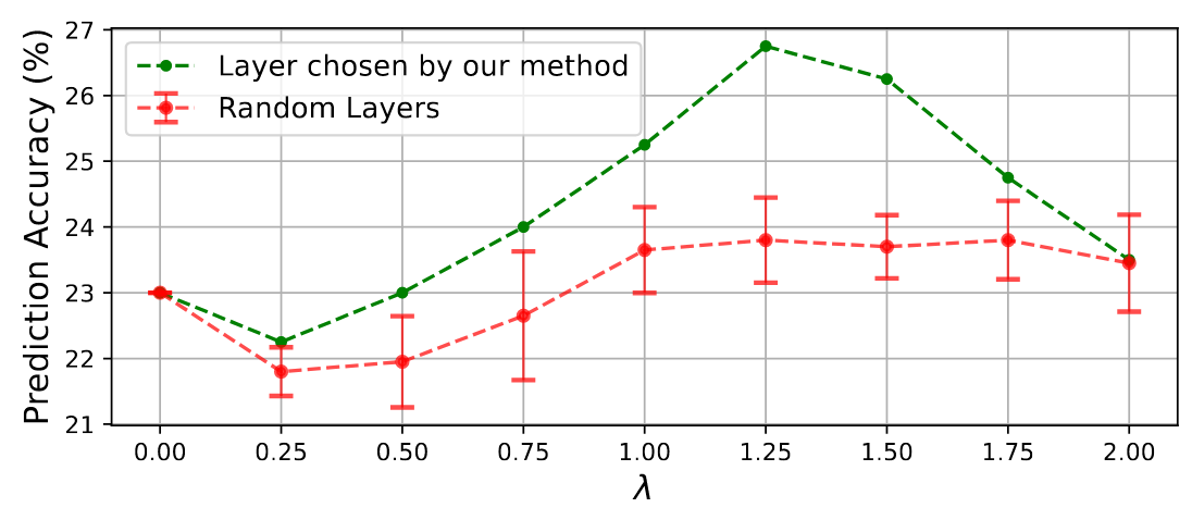
- 아이디어: RQ2에서 관찰한 실패 샘플은 “중간 피크→후반 붕괴”.
- → 그럼 중간의 정보-풍부 레이어 표현을 후반 레이어에 가산(λ 스케일)해 복구해보자(Eq.5).
- 결과:
- 모든 λ 구간에서 제안 방법이 랜덤보다 우위 (오차막대 포함).
- λ 선택 중요: 너무 작거나/크면 비최적, λ=1.25에서 최고.
- 훈련 없이 DeSTA2-Animal에서 상대 16.3% 정확도 향상(λ=0 대비).
- 의미: Layer-wise Information Score로 ‘의미 있는 층’을 골라 후단에 선택적 보강하면, 무학습(post-hoc) 개선 가능.
Test set (400개)에서
\[
h_{-1}^{(\bar{\ell}+5)} \;\leftarrow\;
h_{-1}^{(\bar{\ell}+5)} \;+\; \lambda\, h_{-1}^{(\bar{\ell})}
\]
λ = scaling factor 조절 (1.0~1.5)
My Thoughts
1: Layer-wise Fusion / Adaptive Routing
- 현재 LALM은 encoder→LLM으로 단순 projection을 거치는데,각 층의 정보를 selective하게 결합할 수 있습니다.
- 논문처럼 중간 layer별 attribute-rich representation을 측정한 뒤,
예시
$$ h_{\text{fusion}}^{(\ell)} = \sum_{k \in S} \alpha_k\, h_{\text{audio}}^{(k)} $$
여기서 SSS는 정보 풍부층, α_k는 gating weight (학습 혹은 probing 기반 선택)
→ 이렇게 하면 특정 속성(예: 감정)은 shallow layer,
언어 정보는 deeper layer에서 더 많이 반영하도록 adaptive routing이 가능.
2: Cross-layer Contrastive Alignment
- 즉, “attribute information score”을 일종의 weighting으로 삼아
- cross-modal alignment loss를 가중 적용:
$$
\mathcal{L}_{\mathrm{align}}
= \sum_{\ell} w_{\ell}\,\cdot\,
\operatorname{InfoNCE}\bigl(h_{\mathrm{audio}}^{(\ell)},\, h_{\mathrm{text}}^{(\ell)}\bigr)
$$
오디오 토큰과 텍스트 토큰의 같은 층 에서 나오는 표현 대조학습(InfoNCE)으로 정렬(alignment)
3: Layer-aware Fine-tuning / Adapter Placement
- Layer-wise 정보분포를 미리 측정하면,속성별 정보가 풍부한 층에 집중적으로 배치 가능.
- LoRA/Adapter를 단순히 “중간층에 삽입”하는 것이 아니라
예:
- Emotion → deeper adapter
- Language ID → mid adapter
- Gender → shallow adapter
이렇게 layer-aware tuning 하면 parameter 효율성을 높이면서 성능을 유지·개선 가능.
트랜스포머 레이어별 특징, 붕괴 관련 논문들
- A Closer Look at Multimodal Representation Collapse
- Can VLMs Actually See and Read? A Survey on Modality Collapse in Vision-Language Models
- Multimodal Synthetic Data Finetuning and Model Collapse: Insights from VLMs and Diffusion Models
- When Attention Collapses: How Degenerate Layers in LLMs Enable Smaller, Stronger Models
- Probing Information Distribution in Transformer Architectures through Entropy Analysis